[Must Learning with R_8] ChB1. 기초통계이론 1단계

Wikidocs에 올라와있는 Must Learning with R 을 참고하며 방학동안 부족한 R programming 공부를 하고있습니다.

ChB1. 기초통계이론 1단계

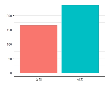
A3. 이항분포(Binomial distribution)

성공확률 0.6인 이항분포 생성

library(ggplot2)

RB = rbinom(n = 400, size =1 ,prob =0.6)
# 난수생성

ggplot(NULL) +
  geom_bar(aes(x = as.factor(RB), fill = as.factor(RB))) +
  theme_bw() +
  xlab("") + ylab("") +
  scale_x_discrete(labels = c("실패", "성공")) +
  theme(legend.position = 'none')

평균과 분산을 수식으로 구현

note that if

$Y \sim Bin(n,p)$,
$P(Y=y) = \begin{pmatrix} n \\ y \end{pmatrix} p^y (1-p), y = 0, 1, 2, \cdots, n$
and $E[Y] = np , Var[Y] = np(1-p)$

library(ggplot2)

#난수생성
X = c()
P = c()


for(k in 1:10){
  
  RDB = dbinom(x = k, size = 10, prob = 0.4)
  
  X = c(X,k)
  P = c(P,RDB)
  
}

ggplot(NULL) +
  geom_bar(aes(x = X, y = P), stat = 'identity') +
  theme_bw() +
  scale_x_continuous(breaks= seq(1,10)) +
  xlab("성공횟수") + ylab("확률")


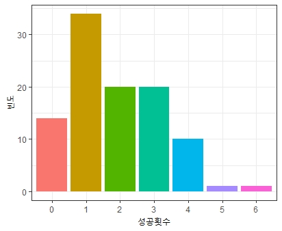
X = c()
P = c()

for(k in 1:10) {
  
  RDB = dbinom(x = k, size = 10, prob = 0.8)
  
  X = c(X,k)
  P = c(P,RDB)
  
}


ggplot(NULL) +
  geom_bar(aes(x = X, y=P), stat = 'identity') +
  theme_bw() +
  scale_x_continuous(breaks = seq(1,10)) +
  xlab("성공횟수")

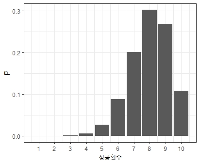
위쪽은 성공확률이 0.4일 때, 성공횟수에 따른 성공확률을 나타내며, 아래쪽은 성공확률이 0.8일 때, 성공횟수에 따른 성공 확률을 의미

A4. 다항분포(multinomial distribution)

RM = as.data.frame(t(rmultinom(n=1, size =10, prob = c(0.2,0.5,0.3))))
RM = colSums(RM)

ggplot(NULL) +
  geom_bar(aes(x = names(RM), y= RM,fill = names(RM)),stat = 'identity') +
  theme_bw() +
  theme(legend.position = 'none') +
  scale_x_discrete(labels = c("1","2","3")) +
  xlab("") + ylab("")

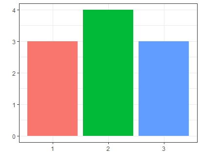
예시)

눈이 3까지 있는 주사위를 10회 던졌을 때,

	1	2	3
확률변수	5개	3개	2개

위 경우의 결과가 나오게 되는 확률을 계산

• pdf를 활용한 계산

  n_F = factorial(10)
  x_F = factorial(5) * factorial(3) * factorial(2)
  Prob = (n_F/ x_F)*(1/3)^5 * (1/3)^3 * (1/3)^2
  Prob
  

  결과

> n_F = factorial(10)
> x_F = factorial(5) * factorial(3) * factorial(2)
> Prob = (n_F/ x_F)*(1/3)^5 * (1/3)^3 * (1/3)^2
> Prob
[1] 0.04267642

• 명령어를 활용한 계산

  dmultinom(c(5,3,2), prob = c(1/3, 1/3, 1/3))
  

  결과

  > dmultinom(c(5,3,2), prob = c(1/3, 1/3, 1/3))
  [1] 0.04267642
  

A5. 포아송분포(Poisson Distribution)

RP = rpois(n = 100, lambda = 2)
RP

ggplot(NULL) +
  geom_bar(aes(x = as.factor(RP), fill = as.factor(RP))) +
  theme_bw() + 
  xlab("성공횟수") + ylab('빈도') +
  theme(legend.position = 'none')

예시)

A도로의 1시간 당 통과 차량 수가 $\lambda=20$인 포아송 분포를 따를 경우, 15대 이하의 차량이 통과할 확률?

ppois(q = 15, lambda = 20, lower.tail = TRUE)

위의 코드는 for $Y \sim Poisson(20)$ 일 때, $P(Y \leq 15)$ 를 의미합니다.

결과

> ppois(q = 15, lambda = 20, lower.tail = TRUE)
[1] 0.1565131

A6. 연속형 확률분포

R = rnorm(n=100000, mean = 0, sd =1)

ggplot(NULL) +
  geom_histogram(aes(x = R, y= ..density..),binwidth = 0.2,fill = "white",col = 'black') +
  geom_density(aes(x = R), col = 'red', size = 1) +
  scale_y_continuous(expand = c(0,0),limits = c(0,0.5)) +
  scale_x_continuous(limits = c(-3,3)) + 
  xlab("") + 
  theme_bw()

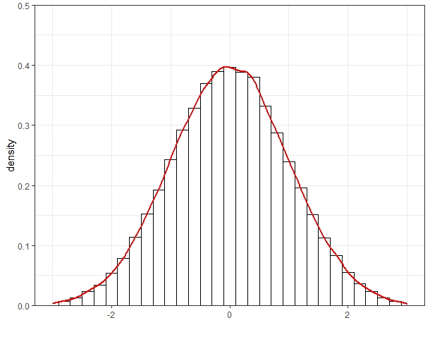
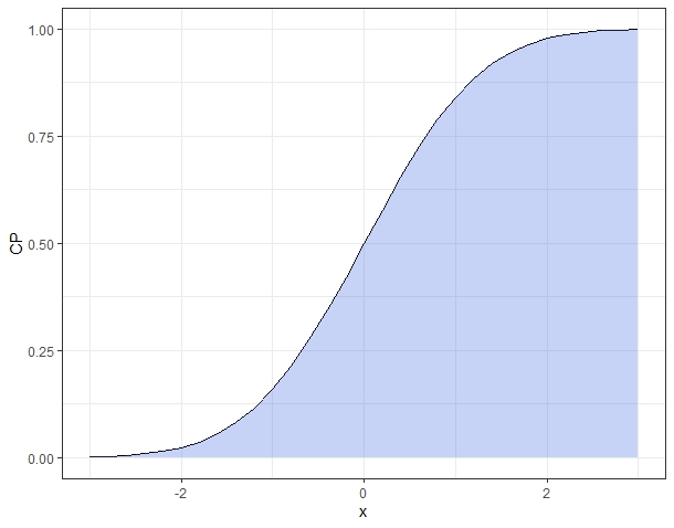
다음과 같은 분포가 있을 때, 위 분포에 대한 누적확률분포는 다음과 같이 구할 수 있다.

CR = ecdf(R) #CDF 계산
x = seq(from = -3, to = 3, by= 0.2)
CP = CR(x)

ggplot(NULL) +
  geom_line(aes(x=x, y=CP)) +
  geom_area(aes(x=x, y=CP), fill = 'royalblue', alpha =0.3) +
  theme_bw()

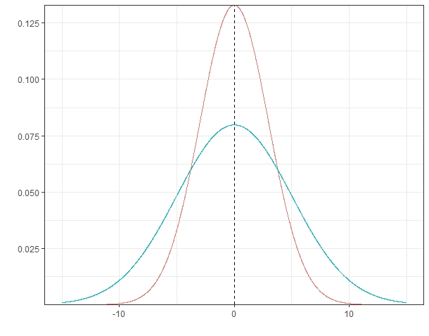
A7. 정규분포(Normal Distribution)

표준편차가 각각 3,5인 정규분포

library(reshape)
library(dplyr)

k1 = c()
p1 = c()

for (k in seq(-15,15,by = 0.01)) {
  
  p = dnorm(x = k, mean = 0, sd =3)
  k1 = c(k1,k)
  p1 = c(p1,p)
  
}


k2 = c()
p2 = c()

for(k in seq(-15,15,by= 0.01)) {
  
  p = dnorm(x = k, mean =0, sd =5)
  k2 = c(k2,k)
  p2 = c(p2,p)
  
}

DF = data.frame(
  k = k1,
  p1= p1,
  p2 = p2
)

DF %>%
  melt(id.vars = c("k")) %>%
  ggplot() +
  geom_line(aes(x = k, y = value, col = as.factor(variable))) +
  geom_vline(xintercept = 0, linetype = 'dashed') +
  theme_bw() +
  theme(legend.position = 'none') +
  xlab("") + ylab("") +
  scale_y_continuous(expand = c(0,0) )